• 1. Preliminary Topics
  • 1.1 Gaussian Distribution
  • 1.2 Jensen’s Inequality
  • 1.3 Matrix Derivatives
• 2.Gaussian Mixture Model (GMM) and Expectation-Maximization(EM) Algorithm
  • 2.1 GMM
  • 2.2 EM
• 3.EM Algorithm for Univariate GMM
  • 3.1 E-Step:
  • 3.2 M-Step:
• 4.EM Algorithm for Multivariate GMM
  • 4.1 E-Step:
  • 4.2 M-Step:
• 5.Summary

1. Preliminary Topics

1.1 Gaussian Distribution

The Gaussian distribution is very widely used to fit random data. The probability density for a one-dimensional random variable $x$ follows:

$$\textit{N}(x; \mu, \sigma) = \frac{1}{\sqrt{2\pi\sigma^2}}\exp\left[-\frac{(x-\mu)^2}{2\sigma^2}\right]$$

where

• $\mu $ is the mean or expectation of the distribution,

• $\sigma$ is the standard deviation, and $ \sigma ^{2}$ is the variance.

More generally, when the data set is a d-dimensional data, it can be fit by a multivariate Gaussian model. The probability density is:

$$\textit{N}(x; \mu, \Sigma) = \frac{1}{\sqrt{(2\pi)^d\det(\Sigma)}}\exp\left[-\frac{1}{2}(x-\mu)^T\Sigma^{-1}(x-\mu)\right]$$

where

• $x$ is a d-by-N vector, representing N sets of d-dimensional random data,
• $\mu$ is a d-by-1 vector, representing the mean of each dimension,
• $\Sigma$ is a d-by-d matrix, representing the covariance matrix

1.2 Jensen’s Inequality

Here statements of Jensen’s inequality in the context of probability theory. These would be used to simplify the target function in an EM process.

Theorem.For convex function $f$ and a random variable $x$:

$$f\left[E(x)\right] \leq E\left[f(x)\right]$$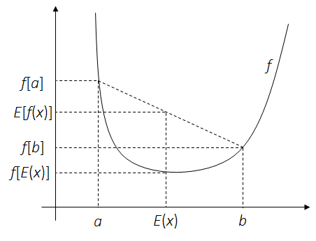

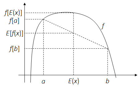
Theorem. For concave function $f$ and a random variable $x$:

$$f\left[E(x)\right] \geq E\left[f(x)\right]$$

1.3 Matrix Derivatives

In order to solve the parameters in a Gaussian mixture model, we need some rules about derivatives of a matrix or a vector. Here are some useful equations cited from The Matrix Cookbook.

$$\begin{aligned} \frac{\partial x^Ta}{\partial x} &= \frac{\partial a^Tx}{\partial x} = a\\ \frac{\partial x^TBx}{\partial x} &= (B + B^T )x\\ \frac{\partial (x -s)^TW(x-s)}{\partial x} &= -2W(x-s), \text{ (W is symmetric)} \\ \frac{\partial a^TXa}{\partial X} &= \frac{\partial a^TX^Ta}{\partial X} = aa^T\\ \frac{\partial \det(X)}{\partial X} &= \det(X)(X^{-1})^T\\ \frac{\partial \ln \det(X)}{\partial X} &= (X^{-1})^T\\ \frac{\partial \det(X^{-1})}{\partial X} &= -\det(X^{-1})(X^{-1})^T\\ \frac{\partial \ln \det(X)}{\partial X^{-1}} &= \frac{\partial \ln \det(X)}{\partial \det(X)}\frac{\partial \det(X)}{\partial X^{-1}} \\ &= \frac{1}{\det(X)}\left[-\det(X)X^T\right]\\ &= -X^T\\ \frac{\partial Tr(AXB)}{\partial X} &= A^TB^T\\ \frac{\partial Tr(AX^-1B)}{\partial X} &= -(X^{-1}BAX^{-1})^T\\ \end{aligned}$$

2.Gaussian Mixture Model (GMM) and Expectation-Maximization(EM) Algorithm

2.1 GMM

For a complex data set in the real-world, it normally consists of a mixture of multiple stochastic processes. Therefore a single Gaussian distribution cannot fit such data set. Instead, a Gaussian mixture model is used to describe a combination of $K$ Gaussian distribution.

Suppose we have a training set of $N$ independent data points $x = {x_1, x_2 …x_i… x_N}$, and the values show multiple peaks. We can model this data set by a Gaussian mixture model

$$p(x|\Theta) = \sum_{k}^{}\alpha_{k}\textit{N}(x; \mu_k, \sigma_k) = \sum_{k}^{}\alpha_{k}\frac{1}{\sqrt{2\pi\sigma_k^2}}\exp\left[-\frac{(x-\mu_k)^2}{2\sigma_k^2}\right]$$

When each data sample $x_i$ is d-dimensional, and the data set $x$ seem scattering to multiple clusters, the data can be modeled by a multivariate version Gaussian mixture model.

$$\begin{aligned} p(x|\Theta) &= \sum_{k}^{}\alpha_{k}\textit{N}(x; \mu_k, \Sigma_k) \\ &= \sum_{k}^{}\alpha_{k}\frac{1}{\sqrt{(2\pi)^d\det(\Sigma_k)}}\exp\left[-\frac{1}{2}(x-\mu_k)^T\Sigma_{k}^{-1}(x-\mu_k)\right] \end{aligned}$$

In the models, $\Theta$ means all parameters, and $\alpha_k$ is the prior probability of th $k^{th}$ Gaussian model, and

$$\sum_{k}\alpha_k = 1$$

2.2 EM

The expectation-maximization(EM) algorithm is an iterative supervised training algorithm. The task is formulated as:

• We have a training set of $N$ independent data points $x$.
• Either we know or have a good guess, that the data set is a mixture of $K$ Gaussian distributions.
• The task is to estimate the GMM parameters: K set of ($\alpha_{k}$, $\mu_k$, $\sigma_k$), or ($\alpha_{k}$, $\mu_k$, $\Sigma_{k}$).

Likelihood Function:

For estimation problems based on data set of independent samples, maximum-likelihood estimation (MLE) is a very widely used and straight forward method to perform estimation.

The probability of N independent tests is described as the product of probability of each test. This is called the likelihood function:

$$p(x|\Theta) = \prod_{i}p(x_i|\Theta)$$

MLE is to estimate the parameters $\Theta$ by maximizing the likelihood function.

$$\Theta = \argmax_{\Theta} \prod_{i}p(x_i|\Theta)$$

By applying the MLE , the likelihood function for uni and multiple variate Gaussian mixture models are very complicated.

$$p(x|\Theta) = \prod_{i}p(x_i|\Theta) = \prod_{i}\left[\sum_{k}\alpha_{k}\textit{N}(x_i| \mu_k, \sigma_k) \right]$$ $$p(x|\Theta) = \prod_{i}p(x_i|\Theta) = \prod_{i}\left[\sum_{k}\alpha_{k}\textit{N}(x_i| \mu_k, \Sigma_k)\right]$$

To estimate K set of Gaussian parameters directly and explicitly is difficult. The EM algorithm simplifies the likelihood function of GMM, and provides an iterative way to optimize the estimation.Here we try to briefly describe the EM algorithm for GMM parameter estimation.

First, the likelihood function of a GMM model can be simplified by taking the log likelihood function. An formula with the form of summation is easier for separating independent data samples and taking derivatives of parameters.

$$L(x|\Theta) = \sum_{i}\ln\left[p(x_{i}|\mu_k, \sigma_k) \right] = \sum_{i}\ln\left[\sum_{k}\alpha_{k}\textit{N}(x_{i}| \mu_k, \sigma_k) \right]$$

Latent Parameters:

There is no efficient way to explicitly maximizing the log likelihood function for GMM above. The EM algorithm introduces a latent parameter $z$, that $z \in {1 ,2 … k … K}$. That is used to describe the probability of a given training sample $x_i$ belonging to cluster z, given full GMM parameters: $p(z|x_{i}, \mu_k, \sigma_k)$

Introduce the latent parameter $z$ in the probability distribution of $x_i$.

$$p(x_{i}|\Theta) = \sum_{k} p(x_{i}|z=k,\mu_k, \sigma_k) p(z=k) \\$$

Compared with $p(x|\Theta) = \sum_{k}^{}\alpha_{k}\textit{N}(x|\mu_k, \sigma_k)$,

we can conclude that $\alpha_k \text{ is the prior probability of } p(z=k)$.

$$p(z=k) = \alpha_k$$

and the conditional probability of $x$ given $z=k$ is the $k^{th}$ Gaussian model.

$$p(x_{i}|z=k,\mu_k, \sigma_k) = \textit{N}(x_i; \mu_k, \sigma_k)$$

Now the latent parameter can be introduced into the log likelihood function. Be noted that an redundant term $p(z|x_{i},\mu_k, \sigma_k) $ is added, in order to match the form of Jensen’s inequality.

$$\begin{aligned} L(x|\Theta) &= \sum_{i}\ln\left[p(x_{i}, z|\mu_k, \sigma_k) \right] \\ &= \sum_{i}\ln \sum_{k} p(x_{i}|z=k, \mu_k, \sigma_k)p(z=k) \\ &= \sum_{i}\ln \sum_{k} p(z=k|x_{i},\mu_k, \sigma_k) \frac{p(x_{i}|z=k, \mu_k, \sigma_k)p(z=k)}{p(z=k|x_{i},\mu_k, \sigma_k)} \\ \end{aligned}$$

Simplify the Likelihood function:

However the summation inside a log function make it difficult to maximize. Here recall Jensen’s inequality:

$$f\left[E(x)\right] \geq E\left[f(x)\right]$$

Let $u$ represent $\frac{p(x_{i} | z=k, \mu_k, \sigma_k)p(z=k)}{p(z | x_{i},\mu_k, \sigma_k)}$ to match Jensen’s inequality.

We get

$$f(u) = \ln u$$ $$E(u) = \sum_{k} p(z|x_{i},\mu_k, \sigma_k) u$$

Therefore,

$$L(x|\Theta) \geq \sum_{i}\sum_{k} p(z=k|x_{i},\mu_k, \sigma_k) \ln \frac{p(x_{i}|z=k, \mu_k, \sigma_k)p(z=k)}{p(z=k|x_{i},\mu_k, \sigma_k)}$$

The posterior probability can be derived by the Bayes’ law.

$$\begin{aligned} p(z=k|x_{i},\mu_k, \sigma_k) &= \frac{ p(x_{i}|z=k,\mu_k, \sigma_k)}{ \sum_{k} p(x_{i}|z=k, \mu_k, \sigma_k)} \\ &= \frac{\alpha_{k}\textit{N}(x_{i}| \mu_k, \sigma_k)}{\sum_{k}\alpha_{k}\textit{N}(x_{i}| \mu_k, \sigma_k)} \end{aligned}$$

Define $\omega_{i,k} = p(z=k|x_{i},\mu_k, \sigma_k) = \frac{\alpha_{k}\textit{N}(x_{i}| \mu_k, \sigma_k)}{\sum_{k}\alpha_{k}\textit{N}(x_{i}| \mu_k, \sigma_k)}$

Then

$$\begin{aligned} L(x|\Theta) &= \sum_{i}\ln \sum_{k} \omega_{i,k} \frac{\alpha_{k}\textit{N}(x_{i}| \mu_k, \sigma_k)}{\omega_{i,k}} \\ &\geq \sum_{i} \sum_{k} \omega_{i,k} \ln\frac{\alpha_{k}\textit{N}(x_{i}| \mu_k, \sigma_k)}{\omega_{i,k}} \end{aligned}$$

This equation defines a lower bound for the log likelihood function. Therefore, an iterative target function for the EM algorithm is defined:

$$Q(\Theta,\Theta^{t}) = \sum_{i}\sum_{k}\omega_{i,k}^t \ln\frac{\alpha_{k}\textit{N}(x_{i}| \mu_k, \sigma_k)}{\omega_{i,k}^t}$$

After $t$ iterations, we’ve got $\Theta^t$，and hence the latent $\omega_{i,k}^t$。 Apply the latest latent parameters in $Q(\Theta,\Theta^{t})$，and then we can update $\Theta^{t+1}$ by maiximization.

Iterative Optimization: 

First the parameters $\Theta$ are initialized, and then $\omega$ and $\Theta$ are updated iteratively.

• After iteration t, a set of parameters $\Theta^t$ have been achieved.

• Calculate latent parameters $\omega_{i,k}^t$ by applying $\Theta^t$ into the GMM. This step is called expectation step.

  $$\omega_{i,k}^t = \frac{\alpha_{k}\textit{N}(x_{i}| \mu_k, \sigma_k)}{\sum_{k}\alpha_{k}\textit{N}(x_{i}| \mu_k, \sigma_k)}$$

• Apply the latest latent parameters $\omega_{i,k}^t$ in the target function. The target function is derived by simplifying the log likelihood funciton by Jensen’s inequality.

  $$Q(\Theta,\Theta^{t}) = \sum_{i}\sum_{k}\omega_{i,k}^t \ln\frac{\alpha_{k}\textit{N}(x_{i}| \mu_k, \sigma_k)}{\omega_{i,k}^t}$$

• With $\omega_{i,k}$, maximize the target log likelihood function, to update GMM parameters $\Theta^{t+1}$. This step is called maximization step.

  $$\Theta^{t+1} = \argmax_{\Theta} \sum_{i}\sum_{k} \ln \omega_{i,k}^t \frac{\alpha_{k}\textit{N}(x_{i}| \mu_k, \sigma_k)}{\omega_{i,k}^t}$$

3.EM Algorithm for Univariate GMM

The complete form of the EM target function for a univariate GMM is

$$Q(\Theta,\Theta^{t}) = \sum_{i}\sum_{k}\omega_{i,k}^t\ln\frac{\alpha_{k}}{\omega_{i,k}^t\sqrt{2\pi\sigma_k^2}}\exp\left[-\frac{(x_i-\mu_k)^2}{2\sigma_k^2}\right]$$

3.1 E-Step:

The E-step is to estimate the latent parameters for each training sample on K Gaussian models. Hence the latent parameter $\omega$ is a N-by-K matrix.

On every iteration, $\omega_{i,k}$ is calculated from the latest Gaussian parameters $(\alpha_k, \mu_k, \sigma_k)$

$$\omega_{i,k}^t = \frac{\alpha_{k}^t\textit{N}(x_{i}| \mu_k^t, \sigma_k^t)}{\sum_{k}\alpha_{k}^t\textit{N}(x_{i}| \mu_k^t, \sigma_k^t)}$$

3.2 M-Step:

$$\Theta := \argmax_{\Theta} Q(\Theta,\Theta^{t})$$

The target likelihood function can be expanded to decouple items clearly.

$$Q(\Theta,\Theta^{t}) = \sum_{i}\sum_{k}\omega_{i,k}^t\left(\ln\alpha_k - \ln \omega_{i,k}^t - \ln \sqrt{2\pi\sigma_k^2}-\frac{(x_i-\mu_k)^2}{2\sigma_k^2}\right)$$

Update $\alpha_k:$

As defined in GMM, $\alpha_k$ is constrained by $\sum_{k}\alpha_k =1$, so estimating $\alpha_k$ is a constrained optimization problem.

$$\begin{gathered} \alpha_k^{t+1} := \argmax_{\alpha_k}{ \sum_{i}\sum_{k}\omega_{i,k}^t\ln\alpha_k}\\ \text{subject to} \sum_{k}\alpha_k =1 \end{gathered}$$

The method of Lagrange multipliers is used to find the local maxima of such constrained optimization problem. We can construct a Lagrangean function:

$$\mathcal{L}(\alpha_k, \lambda) = { \sum_{i}\sum_{k}\omega_{i,k}^t\ln\alpha_k}+ \lambda\left[\sum_{k}\alpha_k -1\right]$$

The local maxima $\alpha_{k}^{t+1}$ should make the derivative of the Lagrangean function equal to 0. Hence,

$$\begin{aligned} \frac{\partial \mathcal{L}(\alpha_k, \lambda) }{\partial \alpha_k} &= { \sum_{i}\omega_{i,k}^t\frac{1}{\alpha_k}}+ \lambda = 0 \\ \Rightarrow \alpha_k &= -\frac{\sum_{i}\omega_{i,k}^t}{\lambda} \end{aligned}$$

By summing the equation for all $k$, the value of $\lambda$ can be calculated.

$$\begin{aligned} \sum_{k}\alpha_k &= -\frac{\sum_{i}\sum_{k}\omega_{i,k}^t}{\lambda} \\ \Rightarrow 1 &= -\sum_{i}\frac{1}{\lambda} = -\frac{N}{\lambda} \\ \Rightarrow \lambda &= -N \end{aligned}$$

Therefore, $\alpha_k$ on iteration $t+1$ based on latent parameters on iteration $t$ is updated by

$$\alpha_k^{t+1} = \frac{\sum_{i}\omega_{i,k}^t}{N}$$

Update $\mu_k:$ 

$\mu_k$ is unconstrained, and can be derived by taking the derivative of the target likelihood function.

$$\mu_k^{t+1} := \argmax_{\mu_k} Q(\Theta,\Theta^{t})$$

Let $\frac{\partial Q(\Theta,\Theta^{t})}{\partial \mu_k}=0$, hence

$$\frac{\partial \sum_{i}\sum_{k}\omega_{i,k}^t\left(\ln\alpha_k - \ln \omega_{i,k}^t - \ln \sqrt{2\pi\sigma_k^2}-\frac{(x_i-\mu_k)^2}{2\sigma_k^2}\right)}{\partial \mu_k} = 0$$ $$\begin{aligned} \sum_{i}\omega_{i,k}^t\frac{x_i-\mu_k}{\sigma_k^2} = 0\\ \Rightarrow \sum_{i}\omega_{i,k}^t\mu_k = \sum_{i}\omega_{i,k}^tx_i \\ \Rightarrow \mu_k\sum_{i}\omega_{i,k}^t = \sum_{i}\omega_{i,k}^tx_i \end{aligned}$$

Hence $\mu_k$ on iteration $t+1$ can be updated as a form of weighted mean of $x$.

$$\mu_k^{t+1} = \frac{\sum_{i}\omega_{i,k}^tx_i}{\sum_{i}\omega_{i,k}^t}$$

Update $\sigma_k:$ 

Similarly, updated $\sigma_k$ is derived by taking the derivative of the target likelihood function with respect to $\sigma_k$.

$$\sigma_k^{t+1} := \argmax_{\sigma_k} Q(\Theta,\Theta^{t})$$

Let

$\frac{\partial Q(\Theta,\Theta^{t})}{\partial \sigma_k} = \frac{\partial \sum_{i}\sum_{k}\omega_{i,k}^t\left(\ln\alpha_k - \ln \omega_{i,k}^t - \ln \sqrt{2\pi\sigma_k^2}-\frac{(x_i-\mu_k)^2}{2\sigma_k^2}\right)}{\partial \sigma_k}=0$.

We get

$$\begin{aligned} \sum_{i}\omega_{i,k}\left[-\frac{1}{\sigma_k}+\frac{(x_i-\mu_k)^2}{\sigma_k^3}\right]&= 0\\ \Rightarrow \sum_{i}\omega_{i,k}\sigma_k^2 &= \sum_{i}\omega_{i,k}(x_i-\mu_k)^2 \\ \Rightarrow \sigma_k^2 \sum_{i}\omega_{i,k} &= \sum_{i}\omega_{i,k}(x_i-\mu_k)^2 \\ \end{aligned}$$

For $\sigma_k$, we can update $\sigma_k^2$, which is enough for Gaussian model calculation. New $sigma_k^2$ depends on $\mu_k$, so normally $\mu_k^{t+1}$ is calculated first and then applied to the update equation for $\sigma_k^2$

$$(\sigma_k^2)^{t+1} = \frac{\sum_{i}\omega_{i,k}(x_i-\mu_k^{t+1})^2 }{\sum_{i}\omega_{i,k}}$$

4.EM Algorithm for Multivariate GMM

Similarlyt the target likelihood function for a multivariat GMM is

$$Q(\Theta,\Theta^{t}) = \sum_{i}\sum_{k}\omega_{i,k}^t\ln\frac{\alpha_{k}}{\omega_{i,k}^t\sqrt{(2\pi)^d\det(\Sigma_k)}}\exp\left[-\frac{1}{2}(x_i-\mu_k)^T\Sigma_k^{-1}(x_i-\mu_k)\right]$$

Be aware that

• $x_i$ is a d-by-1 vecotr,
• $\alpha_k$ is a real number between [0,1],
• $\mu_k$ is a d-by-1 vector,
• $\Sigma_k$ is a d-by-d matrix.
• $\omega$ is a N-by-K matrix.

4.1 E-Step:

The E-step to estimate the latent parameters is the same as univariate GMM, except that the Gaussian distribution is a multivariate one, which is more complicated.

$$\omega_{i,k}^t = \frac{\alpha_{k}^t\textit{N}(x_{i}| \mu_k^t, \Sigma_k^t)}{\sum_{k}\alpha_{k}^t\textit{N}(x_{i}| \mu_k^t, \Sigma_k^t)}$$

The target likelihood function can be expanded.

$$\begin{aligned} &Q(\Theta,\Theta^{t}) \\ &= \sum_{i}\sum_{k}\omega_{i,k}^t\left(\ln\alpha_k - \ln \omega_{i,k}^t - \frac{d}{2}\ln \sqrt{(2\pi)^d} -\frac{1}{2}\ln\det(\Sigma_k)-\frac{1}{2}(x_i-\mu_k)^T\Sigma_k^{-1}(x_i-\mu_k)\right) \end{aligned}$$

4.2 M-Step:

Update $\alpha_{k}:$

The formula to update $\alpha_k$ for multivariate GMMs is exactly the same as univariate GMMs.

$$\begin{gathered} \alpha_k^{t+1} := \argmax_{\alpha_k}{ \sum_{i}\sum_{k}\omega_{i,k}^t\ln\alpha_k}\\ \text{subject to} \sum_{k}\alpha_k =1 \end{gathered}$$

Hence we get the same update equation.

$$\alpha_k^{t+1} = \frac{\sum_{i}\omega_{i,k}^t}{N}$$

Update $\mu_k:$

$$\mu_k^{t+1} := \argmax_{\mu_k} Q(\Theta,\Theta^{t})$$

Take the derivative of $Q(\Theta,\Theta^{t})$ with respec to $\mu_k$, we get

$$\frac{\partial Q(\Theta,\Theta^{t})}{\partial \mu_k} = \sum_{i}\omega_{i,k}^t\frac{\partial \left[-\frac{1}{2}(x_i-\mu_k)^T\Sigma_k^{-1}(x_i-\mu_k)\right]}{\partial \mu_k} = 0\\$$

As the covariance matrix $\Sigma_{k}$ is symmetric, the inverse of it is also symmetric. We can apply $\frac{\partial (x -s)^TW(x-s)}{\partial x} = -2W(x-s)$ (see first section) to the partial derivative.

$$\frac{\partial Q(\Theta,\Theta^{t})}{\partial \mu_k} = \sum_{i}\omega_{i,k}^t \Sigma_{k}^{-1}\left(x_i - \mu_k\right) =0$$ $$\Rightarrow \sum_{i}\omega_{i,k}^t x_i= \mu_k\sum_{i}\omega_{i,k}^t$$

Hence $\mu_k$ on iteration $t+1$ is also updated as a form of weighted mean of $x$. However, in this scenario $\mu_k$ is a d-by-1 vector.

$$\mu_k^{t+1} = \frac{\sum_{i}\omega_{i,k}^t x_i}{\sum_{i}\omega_{i,k}^t}$$

Update $\Sigma_k:$

$$\Sigma_k^{t+1} := \argmax_{\Sigma_k} Q(\Theta,\Theta^{t})$$

Let $\frac{\partial Q(\Theta,\Theta^{t})}{\partial \Sigma_k^{-1}} =0$, we get

$$\begin{aligned} \frac{\partial Q(\Theta,\Theta^{t})}{\partial \Sigma_k^{-1}} &= \sum_{i}\omega_{i,k}^t\frac{\partial \left[ -\frac{1}{2}\ln\det(\Sigma_k)-\frac{1}{2}(x_i-\mu_k)^T\Sigma_k^{-1}(x_i-\mu_k)\right]}{\partial \Sigma_k^{-1}} \\ &= -\frac{1}{2} \sum_{i}\omega_{i,k}^t \left[\frac{\partial \ln\det(\Sigma_k)}{\partial \Sigma_k^{-1}}+\frac{\partial (x_i-\mu_k)^T\Sigma_k^{-1}(x_i-\mu_k)}{\partial \Sigma_k^{-1}} \right] \\ &= 0 \end{aligned}$$

By employing $\frac{\partial \ln \det(X)}{\partial X^{-1}} =-X^T $ and $\frac{\partial a^TXa}{\partial X} = aa^T$(see section one) for the symmetric covariance matrix $\Sigma_k$, and find the maxima of $ Q(\Theta,\Theta^{t})$.

$$\frac{\partial Q(\Theta,\Theta^{t})}{\partial \Sigma_k^{-1}} = \frac{1}{2}\sum_{i}\omega_{i,k}^t \left[\Sigma_k - (x_i-\mu_k)(x_i-\mu_k)^T\right] = 0$$

Similarly, we get the update equation for $\Sigma_k$ at iteration $t+1$, and it depends on $\mu_k$. So again $\mu_k^{t+1}$ is calculated first and then applied to the update equation for $\Sigma_k$

$$\Sigma_k^{t+1} = \frac{\sum_{i}\omega_{i,k}^t (x_i-\mu_k^{t+1})(x_i-\mu_k^{t+1})^T }{\sum_{i}\omega_{i,k}^t}$$

5.Summary

	Univariate GMM	Multivariate GMM
Init	$$\alpha_{k}^0, \mu_k^0, \sigma_k^0$$	$$\alpha_{k}^0, \mu_k^0, \Sigma_k^0$$
E-Step	$$\omega_{i,k}^t = \frac{\alpha_{k}^t\textit{N}(x_{i}| \mu_k^t, \sigma_k^t)}{\sum_{k}\alpha_{k}^t\textit{N}(x_{i}| \mu_k^t, \sigma_k^t)}$$	$$\omega_{i,k}^t = \frac{\alpha_{k}^t\textit{N}(x_{i}| \mu_k^t, \Sigma_k^t)}{\sum_{k}\alpha_{k}^t\textit{N}(x_{i}| \mu_k^t, \Sigma_k^t)}$$
M-Step	$$ \begin{aligned} \alpha_k^{t+1} &= \frac{\sum_{i}\omega_{i,k}^t}{N}\\ \mu_k^{t+1} &= \frac{\sum_{i}\omega_{i,k}^t x_i}{\sum_{i}\omega_{i,k}^t}\\ (\sigma_k^2)^{t+1} &= \frac{\sum_{i}\omega_{i,k}^t(x_i-\mu_k^{t+1})^2 }{\sum_{i}\omega_{i,k}^t} \end{aligned} $$	$$ \begin{aligned} \alpha_k^{t+1} &= \frac{\sum_{i}\omega_{i,k}^t}{N}\\ \mu_k^{t+1} &= \frac{\sum_{i}\omega_{i,k}^tx_i}{\sum_{i}\omega_{i,k}^t}\\ \Sigma_k^{t+1} &= \frac{\sum_{i}\omega_{i,k}^t (x_i-\mu_k^{t+1})(x_i-\mu_k^{t+1})^T }{\sum_{i}\omega_{i,k}^t} \end{aligned} $$